---
title: "4 Adv Spatial Viz P1"
---
## 🧩 Learning Goals
By the end of this lesson, you should be able to:
- Understand the basics of a CRS (coordinate reference system)
- Understand and recognize different spatial file types and data types in R
- Implement some of the basic plotting with the `sf` package
- Understand foundation ideas in working with spatial data (aggregating spatial point data to a spatial region, joining spatial data sets)
## Additional Resources
- Spatial Data Science with Applications in R book: [web](https://r-spatial.org/book/)
- Spatial Data Science with R and `terra` Resources: [web]( https://rspatial.org/)
- Leaflet in R Package: [web](https://rstudio.github.io/leaflet/)
- CRAN task view on spatial analysis: [web](https://cran.r-project.org/web/views/Spatial.html)
## Setup
For this activity, create the following directory structure in your portfolio repository under `src/ica` folder:
```markdown
portfolio
└─ src
   └─ ica
      └─ 04_adv_maps
         ├─ code
         │  └─ 04-adv-maps-1-notes.qmd
         ├─ data
         │  └─ ...  ← saving data here during this activity
         └─ figures
            └─ ...  ← saving created maps here during this activity
```
First load required packages.
```{r setup}
# install.packages(
#   "USAboundariesData",
#   repos = "https://ropensci.r-universe.dev",
#   type = "source"
# )
library(USAboundariesData)

loadNamespace("USAboundariesData")
#Install these packages first

# install.packages(c("sf","elevatr","terra","stars","tidycensus"))
# install.packages('devtools')
# devtools::install_github("ropensci/USAboundaries")
# install.packages("USAboundariesData", repos = "https://ropensci.r-universe.dev", type = "source")


library(tidyverse)
library(sf) # tools for working with spatial vector data (GIS functionality, mapping)
library(elevatr) # access to raster elevation maps
library(terra)
library(stars)
library(tidycensus) # spatial data for the US with census information
library(USAboundaries) # access to boundaries for US states, counties, zip codes, and congressional districts
```
## Spatial Data in R
See [Spatial Data Appendix](https://hash-mac.github.io/stat212site-sp26/notes/spatial-data.html) for basics of CRS and spatial data types.
### Download Shapefiles
1. Navigate to the following URLs to download the spatial data files we'll be using in this activity. Put these files in the `data` folder of your `04_adv_maps` folder.
- MN cities: <https://gisdata.mn.gov/dataset/loc-pop-centers>
- File type: shapefile (`.shp`)
- File name: `shp_loc_pop_centers.zip` (Unzip this after downloading.)
- MN water: <https://gisdata.mn.gov/dataset/us-mn-state-metc-water-lakes-rivers>
- File type: shapefile (`.shp`)
- File name: `shp_water_lakes_rivers.zip` (Unzip this after downloading.)
### Read in Files
2. Read in the MN cities and MN water shapefiles by entering the correct relative paths in `st_read()`. **Tab completion will be very helpful here: type part of a directory or file name and hit tab to autocomplete or bring up a dropdown of options.**
```{r reading}
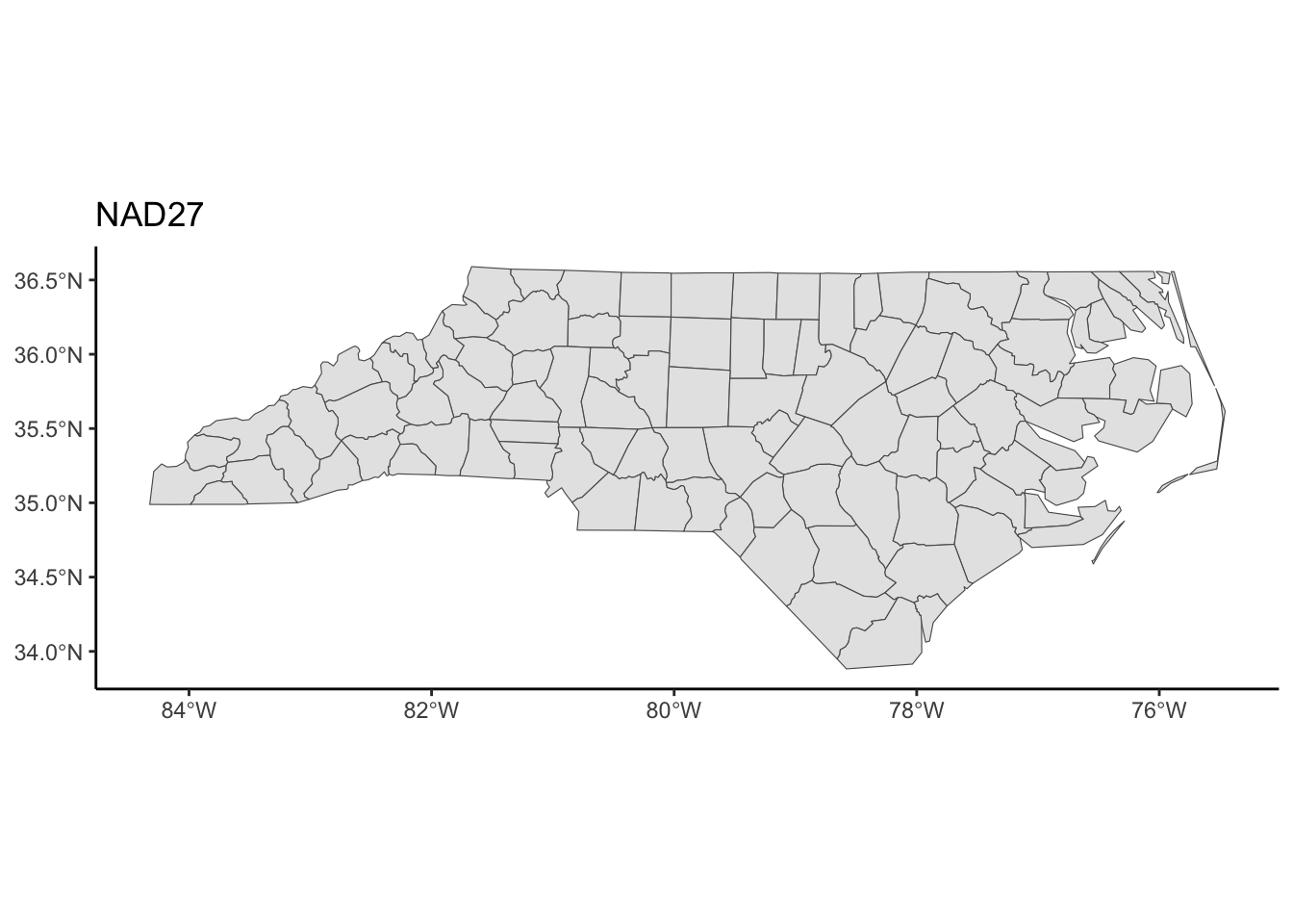
# The sf package comes with a North Carolina shapefile:
nc <- st_read(system.file("shape/nc.shp", package = "sf"))
# Read in shapefiles just downloaded
mn_cities <- st_read("../data/shp_loc_pop_centers/city_and_township_population_centers.shp")
mn_water <- st_read("../data/shp_water_lakes_rivers/LakesAndRivers.shp")
```
The `sf` package reads in spatial data in `data.frame`-like format. Using the `class()` function we can check the **class** (type) of object that we just read in. Note the presence of the "sf" and "data.frame" classes:
```{r check_class_sf}
class(nc)
class(mn_cities)
class(mn_water)
```
When we read in spatial objects, it is useful to check what CRS underlies the data. We can do that with `st_crs()` from the `sf` package:
```{r check_nc_crs}
st_crs(nc)
```
We can treat `sf` objects similarly to ordinary datasets when using `ggplot2` to make spatial visualizations:
```{r nc_first_map}
ggplot(nc) +
    geom_sf() +
    theme_classic() +
    labs(title = "NAD27")
```
### Change CRS
3. Let's explore how changing the CRS changes the map. The `st_transform()` function in `sf` re-expresses a spatial object using a user-supplied CRS. The `crs` argument takes a string descriptor of the CRS. We can find these descriptors via <https://epsg.io>. In the example below, I searched for "South Carolina".
```{r transform_nc}
nc_transformed <- nc |> st_transform(crs = "EPSG:32133")
st_crs(nc_transformed)
ggplot(nc_transformed) +
    geom_sf() +
    theme_classic()
```
The goal is to use <https://epsg.io> to **find two CRSs** that result in a North Carolina map that is noticeably different from the original in the NAD27 CRS.
Take a look at the **function** below that re-maps a spatial object using a new CRS.
- Read through the function to get a sense for how this code works.
- `spatial_obj` and `new_crs` are called **arguments** (function **inputs**).
- Add one more argument called `title` to this function. Use this input to set the plot title.
- Use your function to make two new maps using your chosen CRSs.
```{r transform_via_function}
nc <- st_read(system.file("shape/nc.shp", package = "sf"))
transform_and_plot <- function(spatial_obj, new_crs, title) {
    spatial_obj |>
        st_transform(crs = new_crs) |>
        ggplot() +
            geom_sf() +
            labs(title = title) +
            theme_classic()
}

ggplot(nc) +
    geom_sf() +
    theme_classic() +
    labs(title = "NAD27 (Original)")
transform_and_plot(nc, new_crs = "EPSG:3112", title = "Australia (GDA94)")
transform_and_plot(nc, new_crs = "EPSG:20353", title = "Australia (Queensland, South, West)")
transform_and_plot(nc, new_crs = "EPSG:5940", title = "Russia")
```
**Verify your understanding:** If you had point location data that was not in the NAD27 CRS, what would you expect about the accuracy of how they would be overlaid on the original North Carolina map?
## MN Map with Multiple Layers
**Goal:** create a map of MN with different layers of information (city point locations, county polygon boundaries, rivers as lines and polygons, and a raster elevation map).
### Get County Boundaries
4. We've already read in city location and water information from external shapefiles. We can access county boundaries with the `us_counties()` function in the `USAboundaries` package.
```{r read_county_data}
# Load country boundaries data as sf object
mn_counties <- USAboundaries::us_counties(resolution = "high", states = "Minnesota")

# Take care of duplicate column names (there are two identical "state_name" columns)
names_counties <- names(mn_counties)
names(mn_counties)[names_counties == "state_name"] <- c("state_name1", "state_name2")
```
### Unifying CRSs Across Different Spatial Datasets
5. We first need to ensure that the CRS is the same for all spatial datasets.
- Check the CRS for the `mn_cities`, `mn_water`, and `mn_counties` datasets.
- If the datasets don't all have the same CRS, use `st_transform()` to update the datasets to have the same CRS as `mn_cities`. You can use `crs = st_crs(mn_cities)` within `st_transform()`.
```{r}
# Check CRSs
st_crs(mn_cities)
st_crs(mn_water)
st_crs(mn_counties)
# Transform the CRS of county data to the more local CRS of the cities
mn_counties <- mn_counties |>
    st_transform(crs = st_crs(mn_cities))

# Check the new CRS for mn_counties
st_crs(mn_counties)
```
### Counties + Cities
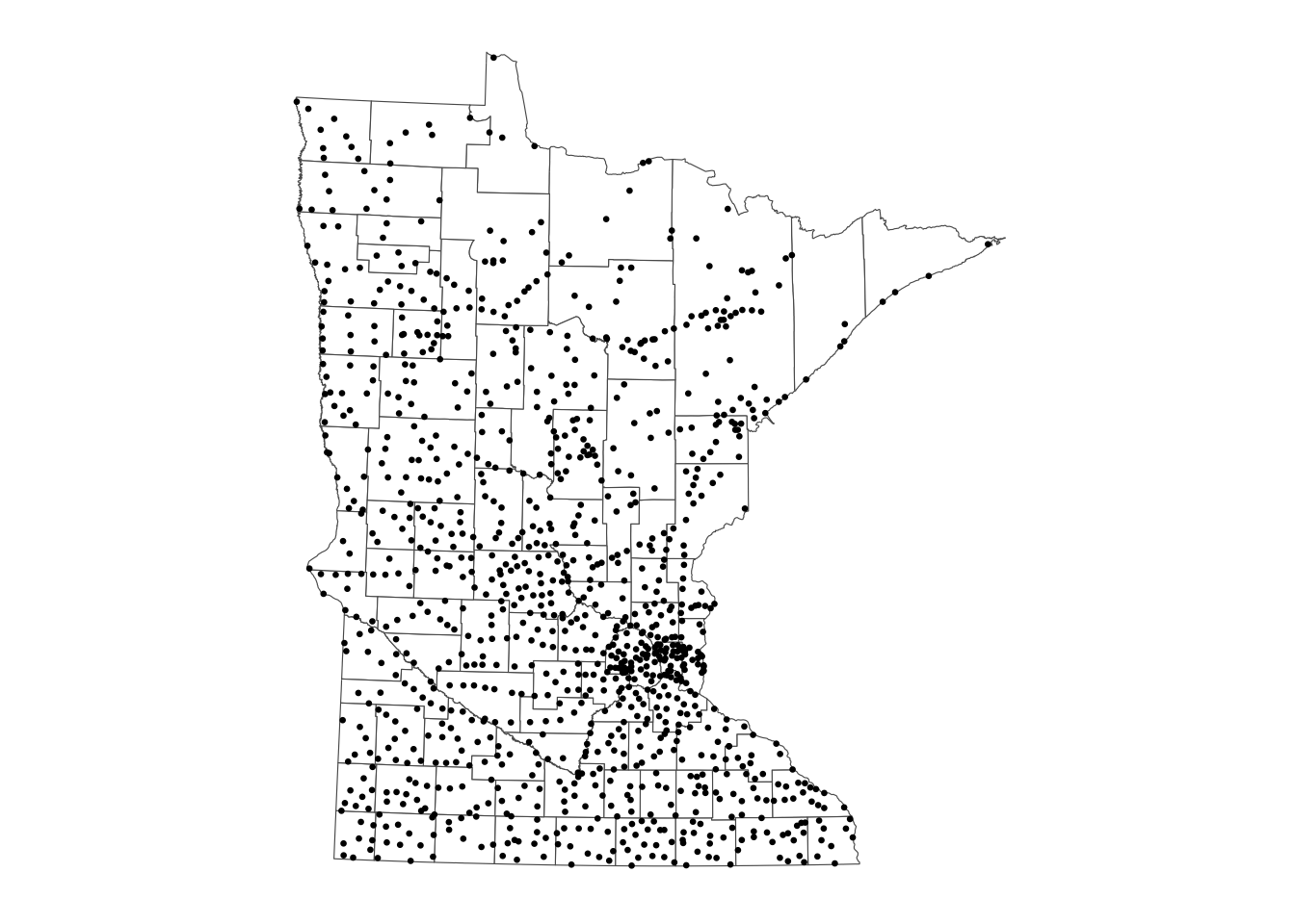
6. Create a map where city locations are overlaid on a map of county boundaries.
- You will need to call `geom_sf()` twice.
- Make the map background white.
- Install the `ggthemes` package, and add the following layer to use a clean map theme: `+ ggthemes::theme_map()`
```{r}
ggplot() +
    geom_sf(data = mn_counties, fill = "white") +
    geom_sf(data = mn_cities, size = 0.5) +
    ggthemes::theme_map()
```
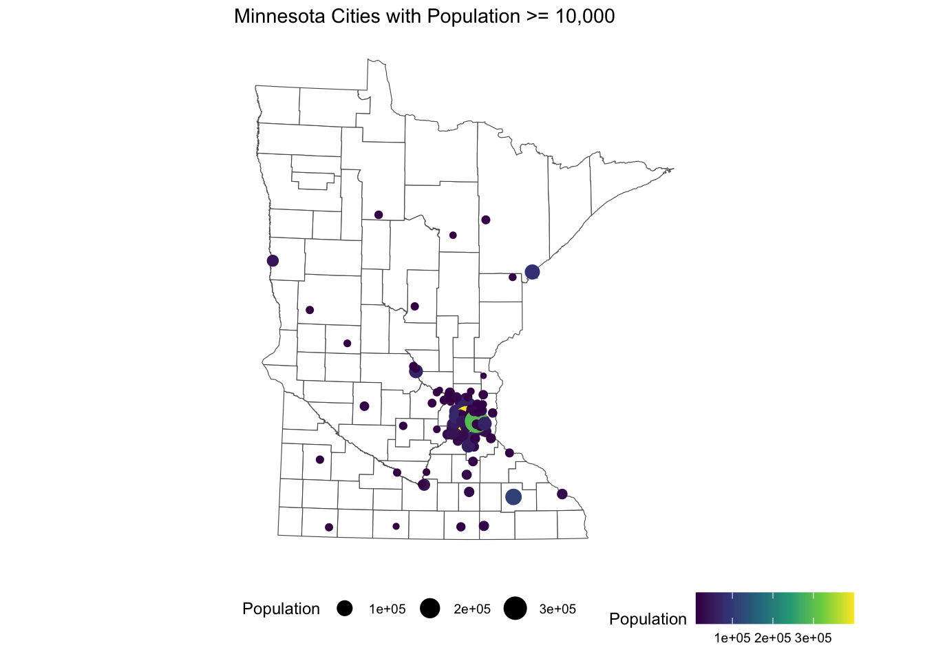
### Customize Colors
7. We can use traditional `ggplot2` aesthetics (e.g., `fill`, `color`) to display location specific attributes. Below we only plot large cities, and we color and size cities according to their population.
```{r mn_map_add_color}
ggplot() +
    geom_sf(data = mn_counties, fill = "white") +
    geom_sf(data = mn_cities |> filter(Population >= 10000), mapping = aes(color = Population, size = Population)) + # cities layer
    scale_color_viridis_c() + # continuous (gradient) color scale
    labs(title = "Minnesota Cities with Population >= 10,000") +
    ggthemes::theme_map() +
    theme(legend.position = "bottom") # move legend
```
Look up the `scale_color_viridis_c()` documentation via the [ggplot2 reference](https://ggplot2.tidyverse.org/reference/scale_viridis.html).
- Read the function description at the top. What is the advantage of using this function for making color palettes?
- Look through the examples section. What is the difference between the `_d()`, `_c()`, and `_b()` variants of this function?
The viridis color scale results in plots that can be interpreted analogously whether in color or black and white and is color-blind friendly.
- The _d() variant is used when color is mapped to a discrete (categorical) variable.
- The _c() variant is used when color is mapped to a continuous variable.
- The _b() variant is used when color is mapped to a continuous variable but when we want that continuous variable to be binned so that there is a small set of colors.
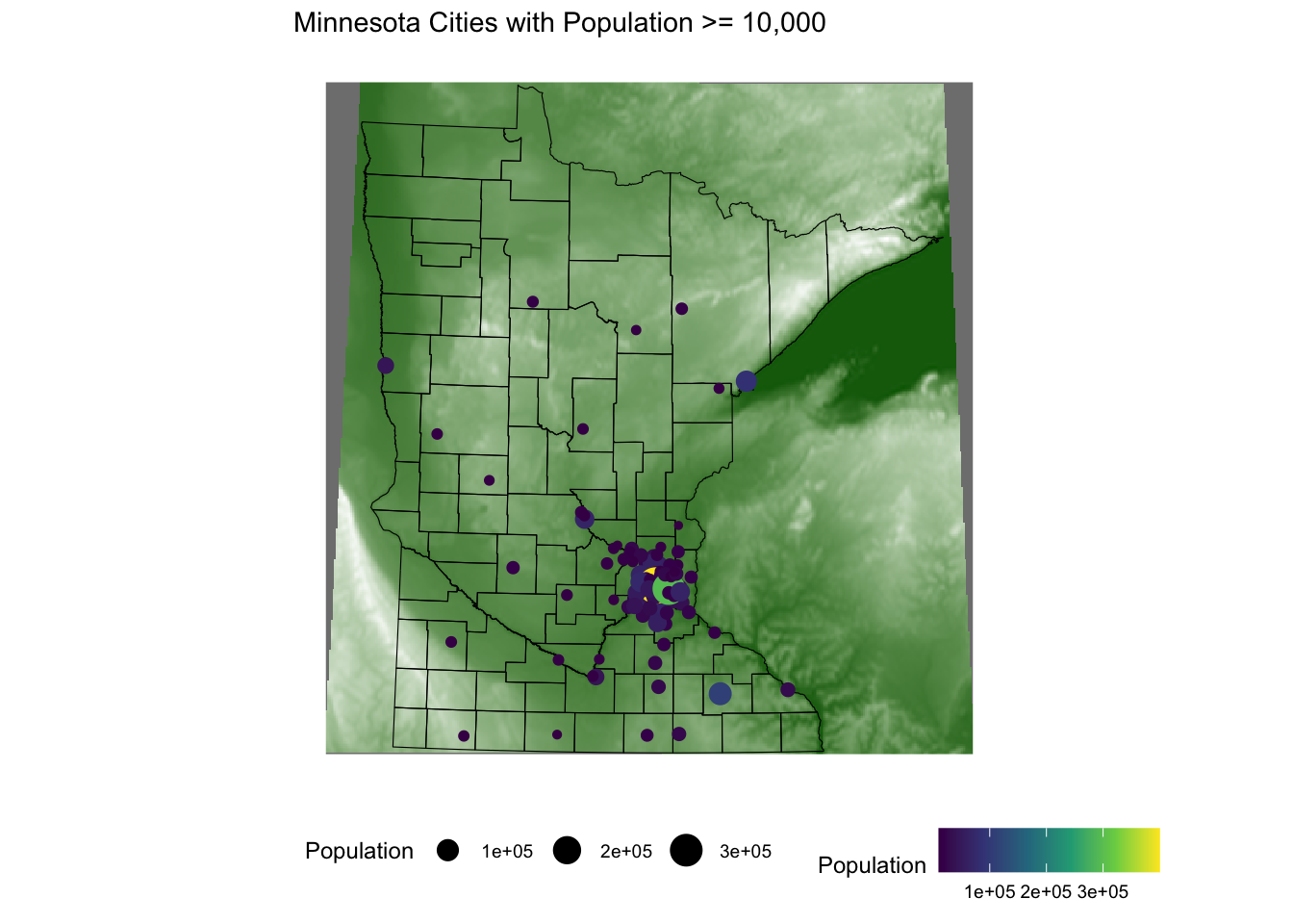
### Adding Elevation Raster Data
Where are large cities located? Is there some relationship to local geography/terrain?
8. To investigate these questions, we can obtain elevation data to include on the map using the `elevatr` package. We encounter two new functions here---we can look up their documentation to make sense of the code by entering the following in the Console:
- `?elevatr::get_elev_raster`
- `?terra::as.data.frame`
```{r get_elevation_data_zoom_out}
elevation <- elevatr::get_elev_raster(mn_counties, z = 5, clip = "bbox")
raster::crs(elevation) <- sf::st_crs(mn_counties)

# Convert to data frame for plotting
elev_df <- elevation |> terra::as.data.frame(xy = TRUE)
colnames(elev_df) <- c("x", "y", "elevation")
```
Build on our existing map by adding a raster layer for elevation as the background.
- Look up the documentation for `geom_raster()` to plot the elevation data from `elev_df`. This will be the first layer of the plot.
- Look at the documentation for `scale_fill_gradient()` to add the following elevation color scale: `"darkgreen"` represents the lowest elevations, and `"white"` represents the highest elevations.
- Add in the layers from the map above to show the largest cities and the county outlines. To remove a background color, use `fill = NA`.
```{r}
ggplot() +
    geom_raster(data = elev_df, aes(x = x, y = y, fill = elevation)) +
    scale_fill_gradient(low = "darkgreen", high = "white", guide = FALSE) +
    geom_sf(data = mn_counties, fill = NA, color = "black") +
    geom_sf(data = mn_cities |> filter(Population >= 10000), mapping = aes(color = Population, size = Population))+
    scale_color_viridis_c() +
    labs(title = "Minnesota Cities with Population >= 10,000") +
    ggthemes::theme_map() +
    theme(legend.position = "bottom")
```
### Zoom in to Twin Cities and Add Water
9. The bulk of the interesting information in this map is in the Twin Cities area. Let's zoom in to this area.
- We can use the `st_bbox()` function to get the **bounding box** for a spatial object---we do this after filtering to the 7 counties in the Twin Cities.
- We then use `st_crop()` to trim a spatial object to a given bounding box.
```{r get_elevation_data_zoom_in}
seven_countyarea <- mn_counties |>
    filter(name %in% c("Anoka", "Hennepin", "Ramsey", "Dakota", "Carver", "Washington", "Scott")) |>
    st_bbox()
seven_countyarea
elevation <- elevatr::get_elev_raster(mn_counties |> st_crop(seven_countyarea), z = 9, clip = "bbox")
raster::crs(elevation) <- sf::st_crs(mn_counties)

# Convert to data frame for plotting
elev_df <- elevation |> terra::as.data.frame(xy = TRUE)
colnames(elev_df) <- c("x", "y", "elevation")
```
In the plot below, we add a layer for water information and a `coord_sf()` layer to restrict the x and y-axis limits to the Twin Cities bounding box. (Without this layer, the map would zoom back out to show all counties and bodies of water).
```{r elevation_map_zoom_in}
png("../figures/tc_map_zoom.png", width = 800, height = 500)
ggplot() +
    geom_raster(data = elev_df, aes(x = x, y = y, fill = elevation)) +
    geom_sf(data = mn_counties, fill = NA, color = "black") + # county boundary layer
    geom_sf(data = mn_water, fill = "lightsteelblue1", color = "lightsteelblue1") + # NEW: river/lake layer
    geom_sf(data = mn_cities |> filter(Population >= 10000), mapping = aes(color = Population, size = Population)) + # cities layer
    scale_color_viridis_c(option = "magma") + # continuous (gradient) color scale
    scale_fill_gradient(low = "darkgreen", high = "white") + # continuous (gradient) fill scale
    coord_sf(xlim = seven_countyarea[c("xmin", "xmax")], ylim = seven_countyarea[c("ymin", "ymax")]) + # NEW: crop map to Twin Cities bounding box
    labs(title = "Twin Cities with Population >= 10,000") +
    ggthemes::theme_map() +
    theme(legend.position = "none") # remove legend
dev.off()
```
Let's add to the above code chunk to save the map above to an image file called `tc_map_zoom.png` in the `figures` folder. The code example below shows a general template for saving a plot to file. Choose a reasonable width and height. (There are also `jpeg()` and `pdf()` functions for writing images.)
```{r save_plot_example, eval=FALSE}
# png("../figures/tc_map_zoom.png", width = 800, height = 500)
# # Code for creating plot
# dev.off()
```
## Going Beyond - Twin Cities Map with `leaflet`
Below we show how to make the MN counties map in the `leaflet` package.
```{r leaflet}
library(leaflet)

mn_counties_leaf <- mn_counties |> st_transform(4326) # Leaflet expects this CRS for vectors
mn_cities_leaf <- mn_cities |> st_transform(4326)

cities_per_county <- st_join(mn_cities_leaf, mn_counties_leaf) |>
    st_drop_geometry() |> # removes geometry - makes the following calculation more efficient
    count(name)

mn_counties_leaf |>
    filter(name %in% c("Anoka", "Hennepin", "Ramsey", "Dakota", "Carver", "Washington", "Scott")) |>
    left_join(cities_per_county) |>
    leaflet() |>
    addProviderTiles("CartoDB.Positron") |>
    addPolygons(
        color = "#444444", weight = 1, smoothFactor = 0.5, opacity = 1.0,
        fillOpacity = 0.5, fillColor = ~colorQuantile("YlOrRd", n)(n),
        highlightOptions = highlightOptions(color = "white", weight = 2, bringToFront = TRUE)) |>
    addCircles(data = mn_cities_leaf |> filter(County %in% paste(c("Anoka", "Hennepin", "Ramsey", "Dakota", "Carver", "Washington", "Scott"), "County")), color = "#444444")
```
## Done!
- Check the ICA Instructions for how to (a) push your code to GitHub and (b) update your portfolio website