Member 2 Nox Matse
Your exploratory data analysis of the team datasets go here.
  Year       Player.Name Position Team  College...Origin Year.Drafted
1 1997  Adrienne Johnson        G  CLE        Ohio State         1999
2 1997 Andrea Congreaves      F-C  CHA Mercer University         1997
3 1997    Andrea Stinson        G  CHA          NC State         1997
4 1997     Anita Maxwell        F  CLE  New Mexico State         1997
5 1997    Bridget Pettis        G  PHO           Florida         1997
6 1997  Bridgette Gordon        F  SAC         Tennessee         1997
  Draft.Pick Height Weight Minutes.Per.Game Points.Per.Game Rebounds.Per.Game
1          8   5-10  154lb              7.8             2.1               0.9
2         26    6-2  183lb             23.5             6.7               4.8
3              5-10  158lb             36.1            15.7               5.5
4         29                            7.0             2.1               1.3
5          7    5-9                    30.1            12.6               3.8
6               6-0  172lb             35.0            13.0               4.8
  Assists.Per.Game Blocks.Per.Game Steals.Per.Game Turnovers.Per.Game   FG.
1              0.4             0.0             0.2                1.1 0.379
2              1.5             0.2             0.6                1.1 0.500
3              4.4             0.8             1.5                3.5 0.447
4              0.9             0.0             0.4                0.7 0.320
5              2.8             0.4             1.8                2.9 0.334
6              2.8             0.3             1.4                3.0 0.433
   X3P.   FT. Win.Shares
1 0.500 0.778       -0.5
2 0.409 0.768        3.1
3 0.325 0.674        3.8
4    NA 0.375       -0.1
5 0.306 0.898        3.2
6 0.275 0.785        1.9
Code
# library(randomForest)
# library(dplyr)
#
# # Clean and select variables
# wnba_clean <- wnba2 %>%
#   select(Draft.Pick, Points.Per.Game, College...Origin, Win.Shares, Assists.Per.Game, Rebounds.Per.Game, Minutes.Per.Game, Height) %>%
#   na.omit()
#
# # Make sure overall_pick is numeric
# wnba_clean$overall_pick <- as.numeric(wnba_clean$Draft.Pick)
#
# # Train model
# rf_model <- randomForest(
#   Draft.Pick ~ .,
#   data = wnba_clean,
#   importance = TRUE
# )
#
# # View importance
# importance(rf_model)
# varImpPlot(rf_model)
Code
# library(glmnet)
# library(dplyr)
#
# # Clean data
# wnba_clean2 <- wnba2 %>%
#   select(Draft.Pick, Points.Per.Game, College...Origin, Win.Shares, Assists.Per.Game, Rebounds.Per.Game, Minutes.Per.Game, Height) %>%
#   na.omit()
#
# # X and Y
# x <- as.matrix(wnba_clean %>% select(-Draft.Pick))
# y <- wnba_clean$Draft.Pick
#
# # LASSO
# cv_model <- cv.glmnet(x, y, alpha = 1)
# lasso_model <- glmnet(x, y, alpha = 1, lambda = cv_model$lambda.min)
#
# # Convert coefficients to dataframe
# coef_df <- as.matrix(coef(lasso_model)) %>%
#   as.data.frame()
#
# # Rename the coefficient column safely
# colnames(coef_df)[1] <- "coefficient"
#
# # Add variable names + rank
# coef_df <- coef_df %>%
#   mutate(variable = rownames(.)) %>%
#   arrange(desc(abs(coefficient)))
#
# # View results
# coef_df
Code
library(dplyr)
library(glmnet)

# Step 1: clean data
clean_data <- wnba2 %>%
  mutate(
    Draft.Pick = as.character(Draft.Pick),
    Draft.Pick[Draft.Pick %in% c("Undrafted", "")] <- NA,
    Draft.Pick = as.numeric(Draft.Pick)
  ) %>%
  filter(!is.na(Draft.Pick)) %>%
  select(where(is.numeric)) %>%
  na.omit()   # ⚠️ THIS is key: removes any remaining NA rows

# Step 2: create X and y from SAME dataset
x <- model.matrix(Draft.Pick ~ ., clean_data)[, -1]
y <- clean_data$Draft.Pick

# Step 3: run LASSO
cv_model <- cv.glmnet(x, y, alpha = 1)
lasso_model <- glmnet(x, y, alpha = 1, lambda = cv_model$lambda.min)

# Step 4: extract important variables
important_vars <- coef(lasso_model)
important_vars[important_vars != 0]
[1] 449.87417945 -0.21357143 -0.64337016 -0.07384913 -0.13357690
[6] -1.63063561 0.43600870 -1.00145202 1.53330522 -2.02640879
[11] 0.09786055Code
library(dplyr)

coef_df <- as.matrix(coef(lasso_model)) %>%
  as.data.frame()

# Rename column
colnames(coef_df)[1] <- "coefficient"

# Add variable names and clean up
coef_df <- coef_df %>%
  mutate(variable = rownames(.)) %>%
  filter(coefficient != 0) %>%   # keep only important variables
  arrange(desc(abs(coefficient)))

# View
coef_df
coefficient variable
(Intercept) 449.87417945 (Intercept)
FT. -2.02640879 FT.
Blocks.Per.Game -1.63063561 Blocks.Per.Game
X3P. 1.53330522 X3P.
Turnovers.Per.Game -1.00145202 Turnovers.Per.Game
Points.Per.Game -0.64337016 Points.Per.Game
Steals.Per.Game 0.43600870 Steals.Per.Game
Year -0.21357143 Year
Assists.Per.Game -0.13357690 Assists.Per.Game
Win.Shares 0.09786055 Win.Shares
Rebounds.Per.Game -0.07384913 Rebounds.Per.GameCode
library(dplyr)
library(randomForest)

# Step 1: clean data (same logic as before)
clean_data <- wnba2 %>%
  mutate(
    Draft.Pick = as.character(Draft.Pick),
    Draft.Pick[Draft.Pick %in% c("Undrafted", "")] <- NA,
    Draft.Pick = as.numeric(Draft.Pick)
  ) %>%
  filter(!is.na(Draft.Pick)) %>%
  select(where(is.numeric)) %>%
  na.omit()

# Step 2: run random forest
set.seed(123)

rf_model <- randomForest(
  Draft.Pick ~ .,
  data = clean_data,
  importance = TRUE,
  ntree = 500
)

# Step 3: extract variable importance
importance_df <- as.data.frame(importance(rf_model))
importance_df$variable <- rownames(importance_df)

# Sort by importance
importance_df <- importance_df %>%
  arrange(desc(IncNodePurity))

# View results
importance_df
%IncMSE IncNodePurity variable
Points.Per.Game 46.16407 54441.30 Points.Per.Game
Year.Drafted 60.47708 42769.57 Year.Drafted
Minutes.Per.Game 26.22497 37146.72 Minutes.Per.Game
Rebounds.Per.Game 38.46880 28773.92 Rebounds.Per.Game
Year 41.95568 28526.85 Year
Turnovers.Per.Game 36.20875 25126.84 Turnovers.Per.Game
FG. 31.06777 24920.98 FG.
FT. 29.36691 23636.38 FT.
Assists.Per.Game 38.93775 22308.18 Assists.Per.Game
X3P. 28.13583 21756.51 X3P.
Win.Shares 23.59044 21344.32 Win.Shares
Steals.Per.Game 26.44115 16384.42 Steals.Per.Game
Blocks.Per.Game 31.94281 13973.31 Blocks.Per.Game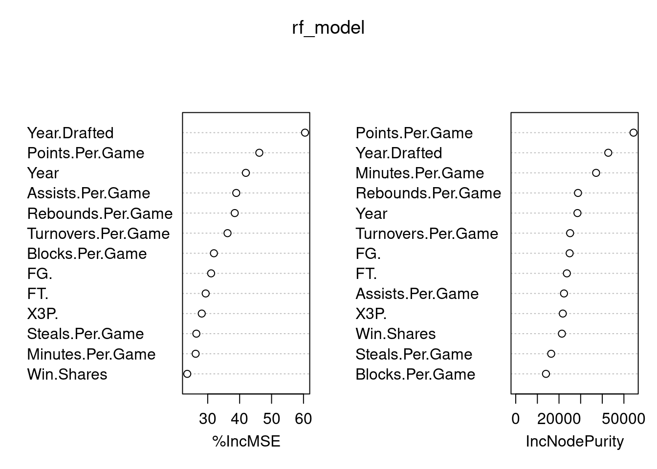
%IncMSE Measures how much prediction error increases if a variable is removed
Higher = more important
IncNodePurity (right plot)
Measures how much a variable improves tree splits
both plots show that points per game, year drafted, year and minutes per minute are important from random forest
Code
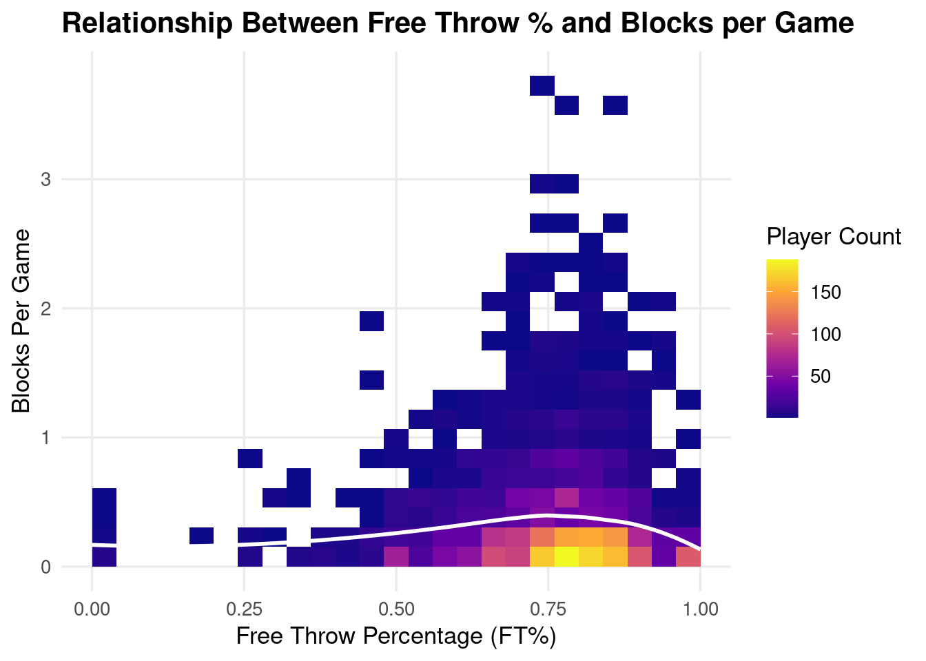
ggplot(clean_data, aes(x = FT., y = Blocks.Per.Game)) +
  geom_bin2d(bins = 25) +
  scale_fill_viridis_c(option = "C") +
  geom_smooth(method = "loess", se = FALSE, color = "white", linewidth = 1) +
  labs(
    title = "Relationship Between Free Throw % and Blocks per Game",
    x = "Free Throw Percentage (FT%)",
    y = "Blocks Per Game",
    fill = "Player Count"
  ) +
  theme_minimal(base_size = 13) +
  theme(
    plot.title = element_text(face = "bold"),
    panel.grid.minor = element_blank()
  )
Code
library(ggplot2)
library(dplyr)
library(tidyr)
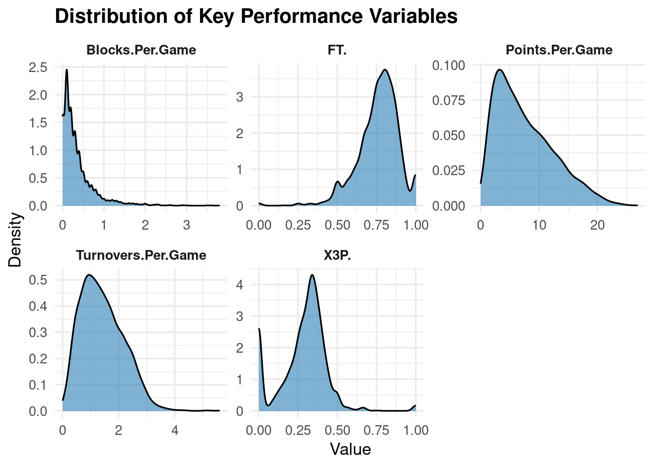
top_vars <- clean_data %>%
select(FT., Blocks.Per.Game, X3P., Turnovers.Per.Game, Points.Per.Game) %>%
pivot_longer(cols = everything(),
names_to = "variable",
values_to = "value")
ggplot(top_vars, aes(x = value)) +
geom_density(fill = "#2C7FB8", alpha = 0.6) +
facet_wrap(~variable, scales = "free") +
labs(
title = "Distribution of Key Performance Variables",
x = "Value",
y = "Density"
) +
theme_minimal(base_size = 13) +
theme(
strip.text = element_text(face = "bold"),
plot.title = element_text(face = "bold")
)