What factors influence success in a WNBA player?

Before we answer that question, let’s go over some motivation.

Motivation

The WNBA Draft is an annual event in which teams select eligible college players and international prospects to join the league, shaping the next generation of professional women’s basketball talent. Similar to other professional sports drafts, selection order is largely determined by the previous season’s standings, with weaker teams given higher picks in an effort to maintain competitive balance. For general managers, the draft represents a critical decision point: players are evaluated not only on traditional box-score statistics such as points, rebounds, and assists, but also on efficiency measures, defensive contributions, and advanced indicators of value like win shares.

In this analysis, we treat the draft as a decision problem where the goal is to identify players who are likely to provide the greatest overall impact at the professional level. Using available collegiate and pre-draft performance metrics—including per-game production, shooting efficiency (field goal, three-point, and free throw percentages), and all-around contributions such as steals, blocks, and turnovers—we aim to build a data-driven framework for player selection. This approach allows us to move beyond draft position alone and systematically compare prospects based on their statistical profiles and projected value to a WNBA roster.

… so why the WNBA?

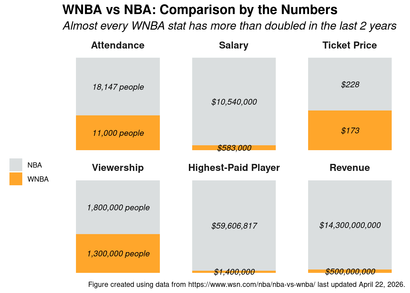
We wanted to understand what factors contribute to a WNBA player succeeding in the league. Given that the WNBA is a newer and more developing league, trends are not as established as they are in the NBA. Does height play a bigger role than weight? Does being selected early in the draft guarantee a more productive career? These are the kinds of questions that motivated us to look more closely at the data the league has generated over its nearly three decades of existence.

This brings us to our research question:

What factors influence the success of a WNBA player?

Data

To answer that question, we assembled a dataset covering every player season recorded in the WNBA from 1997 to 2025

drawing from Basketball Reference as our primary source.

1997-2025

The final dataset contains

across

filtered to players with at least five minutes per game.

1,011 unique players

4,828 player seasons

Each observation captures the following player statistics:

in addition to per game statistics like:

as well as our predictor variable:

Win shares is a single number that attempts to credit each player with a portion of their team’s wins based on both their offensive and defensive contributions. A player averaging around 1.3 win shares in a season is performing near the league median. A player generating 5 or more in a season is among the most impactful in the league that year.

Player Statistics

• year
• position
• team
• university
• country of origin
• draft year
• draft pick
• height
• weight

Per Game Statistics

• points
• rebounds
• assists
• blocks
• steals
• turnovers
• shooting percentages

Win Shares

To explore the data visually, we examined how win shares are distributed across the full dataset, how they vary by position and era, and how individual statistics relate to overall contributions. We built several regression models ranging from a standard OLS regression on performance statistics, to a physical attributes only model, to a combined model, and finally a random forest to capture nonlinear structure and rank feature importance across all predictors simultaneously.

Results

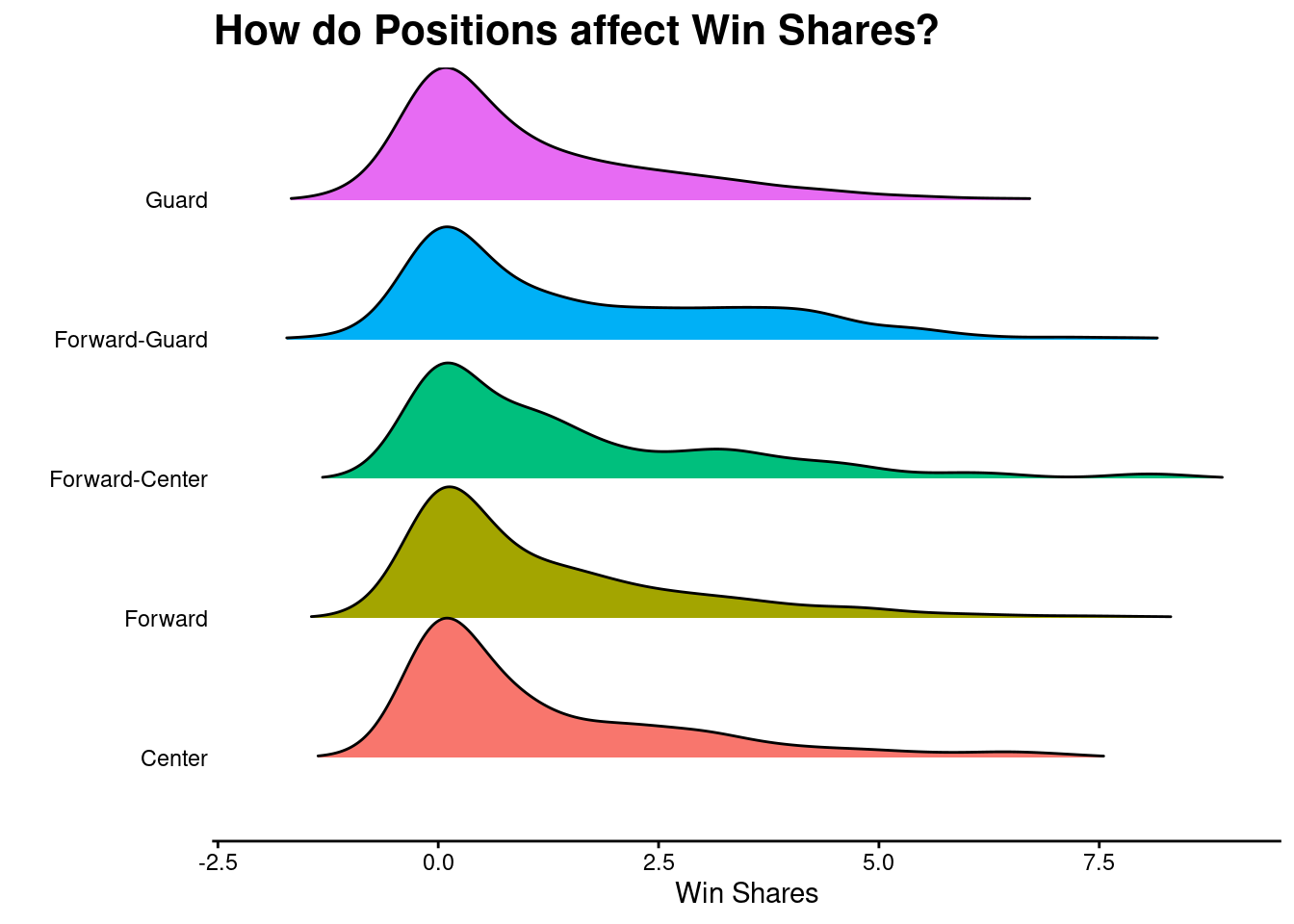
One thing we looked at was player positions. Specifically, how player position was related to a player’s win shares.

What we found was that all positions tend to have relatively similar effects on win shares…

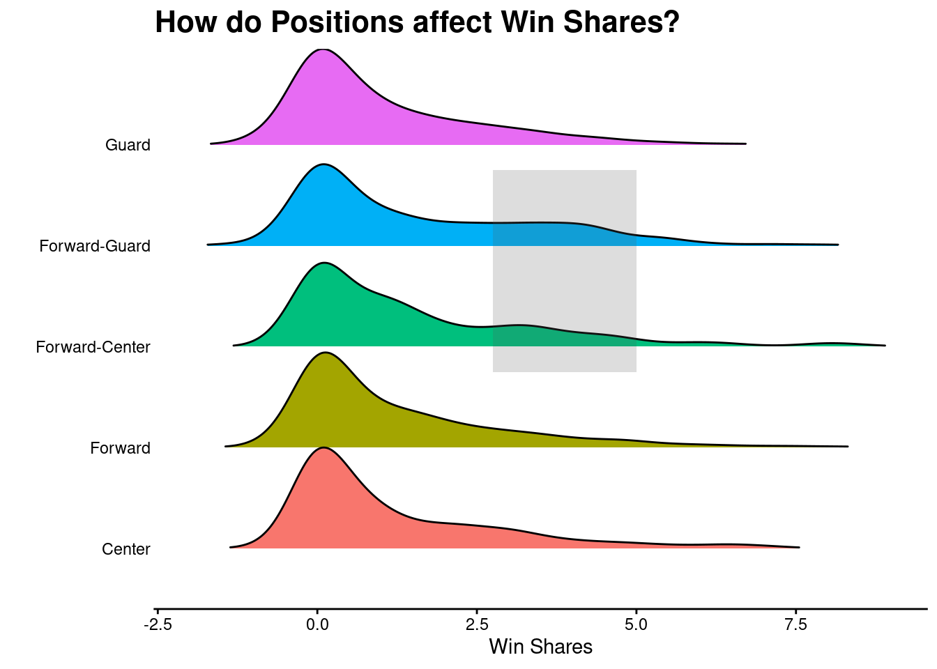
…however, players that can play multiple positions can also have higher win shares

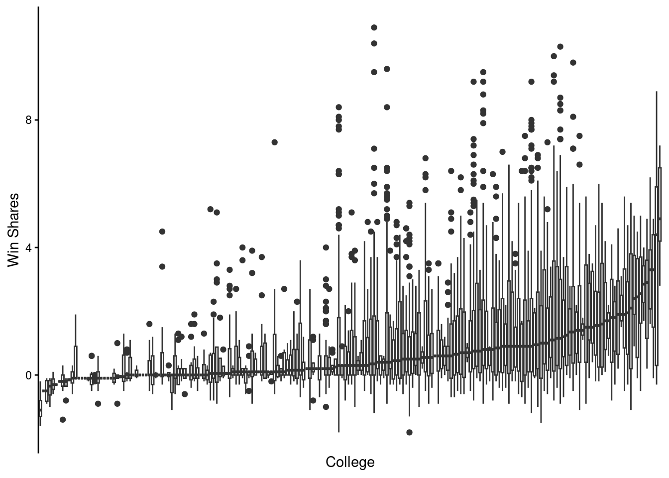
Perhaps there are specific schools that produce stellar players?

In fact, there are.

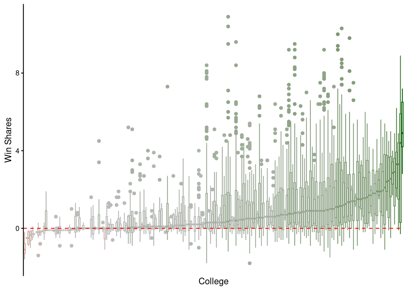
However, most school actually produce good players.

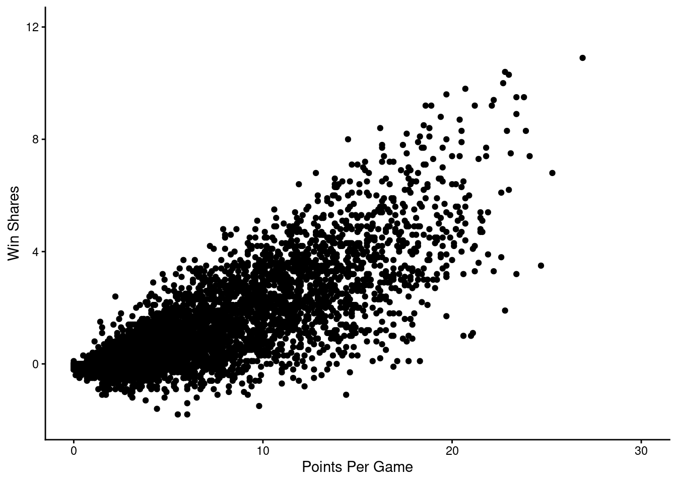
Based on intuition alone, we’d expect players that score more points to contribute the most to win shares.

That intuition turns out to be correct…

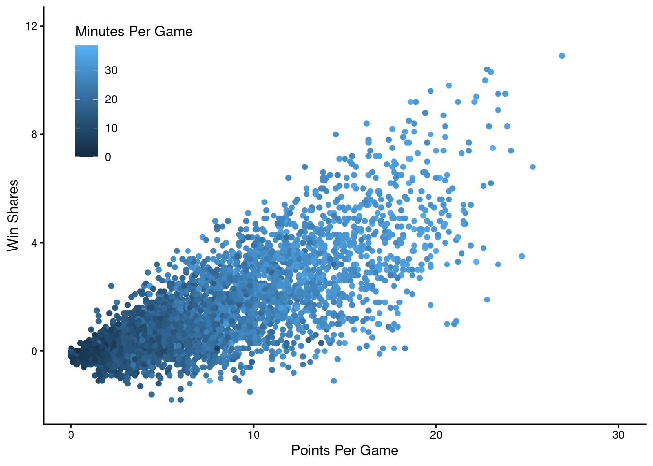
and closely related to minutes per game, where players that play longer tend to score more points (and vice versa), which improves a player’s Win Shares.

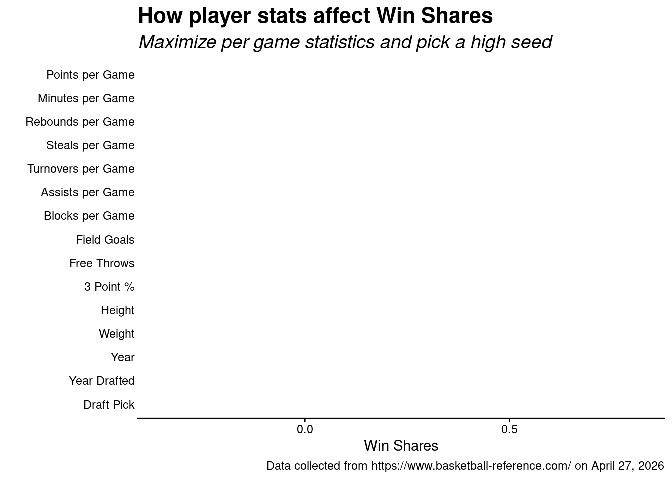
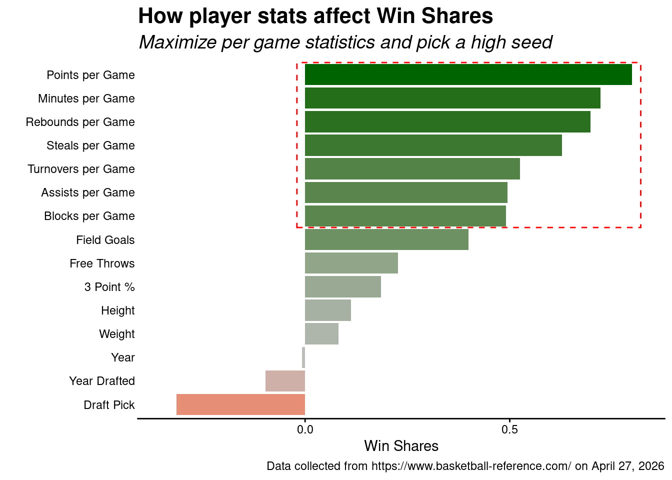
When we look at all numeric variables…

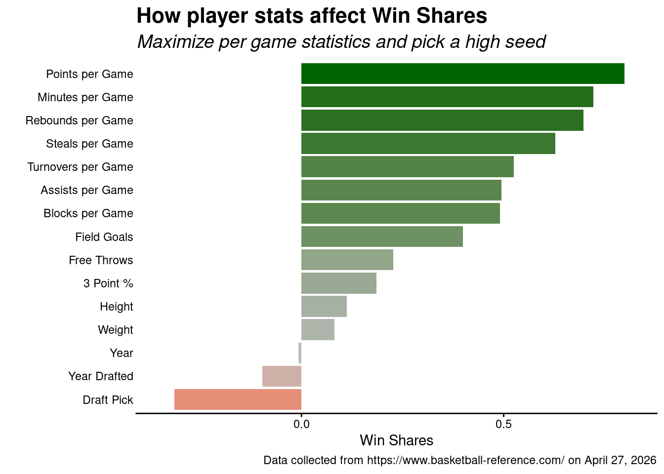
…we see that being proficent in nearly any of them would make you a more valuable player…

…however, players that can maximize their per-game statistics tend to be more valuable players on the court.

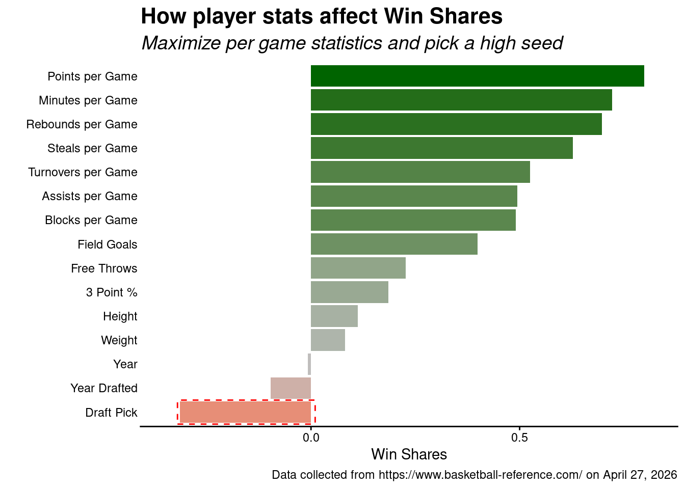
Additionally, if you can minimize your draft pick number – that it, be a number close to 1 (i.e., be first pick) – you tend to do well in terms of win shares.

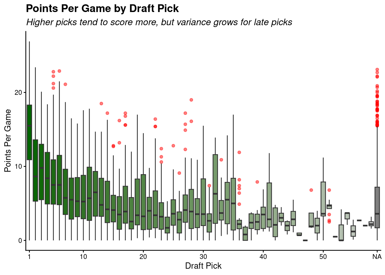
Speaking of draft pick…

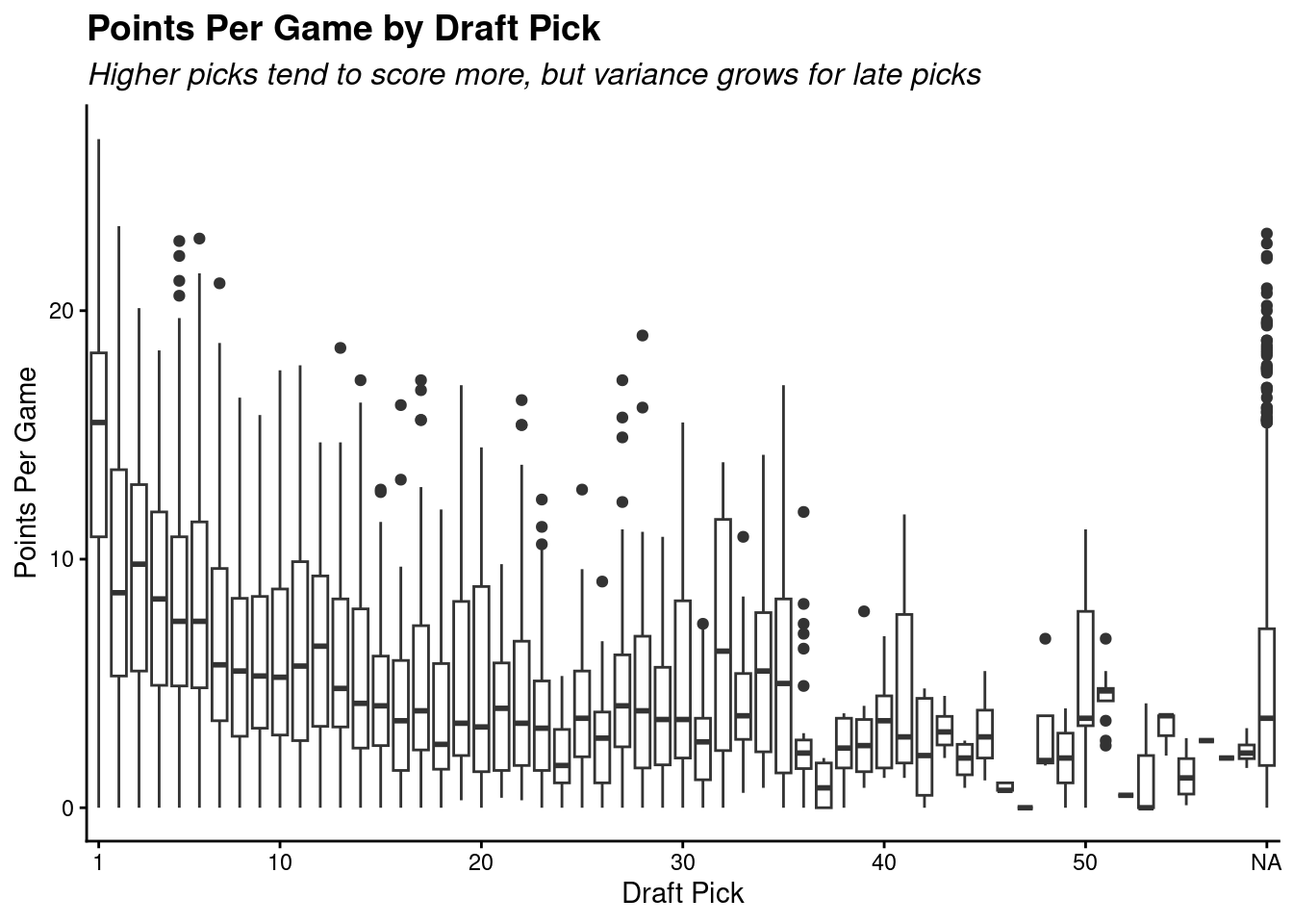
This graph illustrates the points-per-game scoring from each draft pick slot across all years of our dataset.

Higher picks score, on average, more points per game than players of lower draft slots. A notable difference is that the NA category is very widespread in its outcomes. This is due to undrafted free agents and international players who were not formally drafted, but were successful anyways.

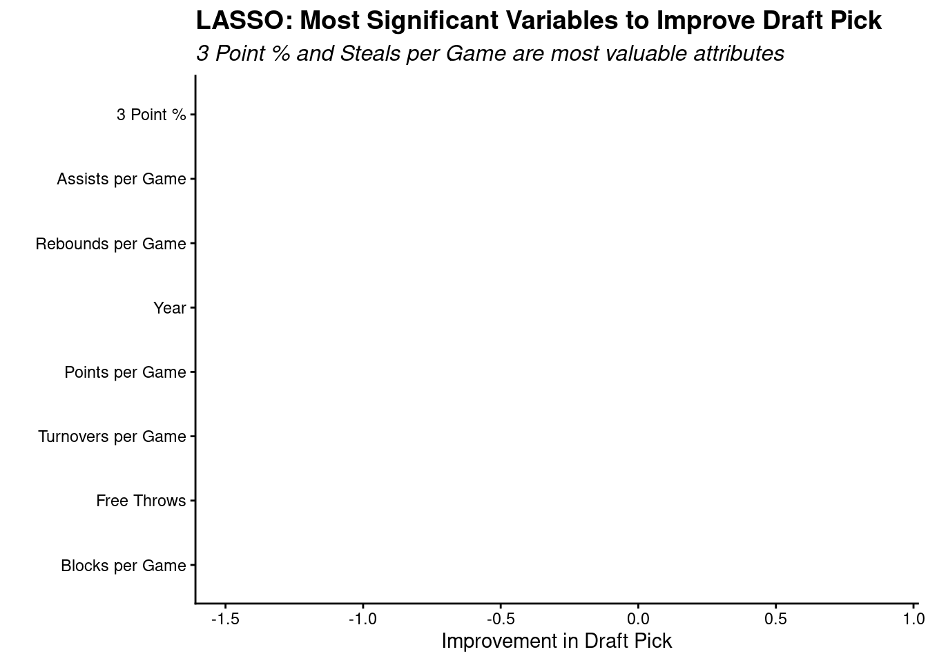
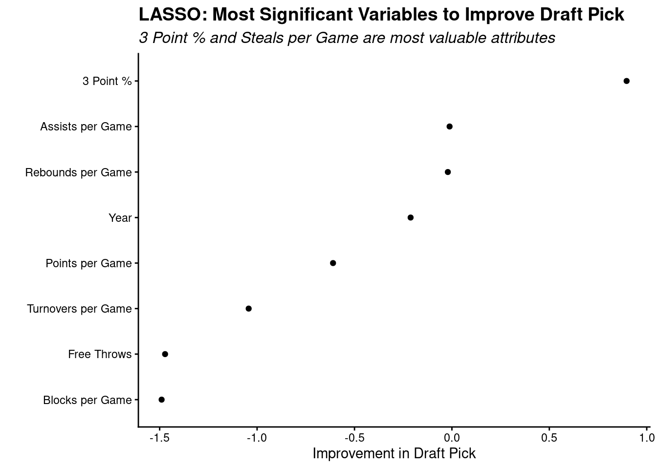
When we look at the most significant variables that effect a player’s draft pick, through a LASSO model…

…we see the percentage of 3-pointers is most important according to the LASSO model. Although still a variable to be considered, the free throws are not a meaningful variable to look at for draft selection.

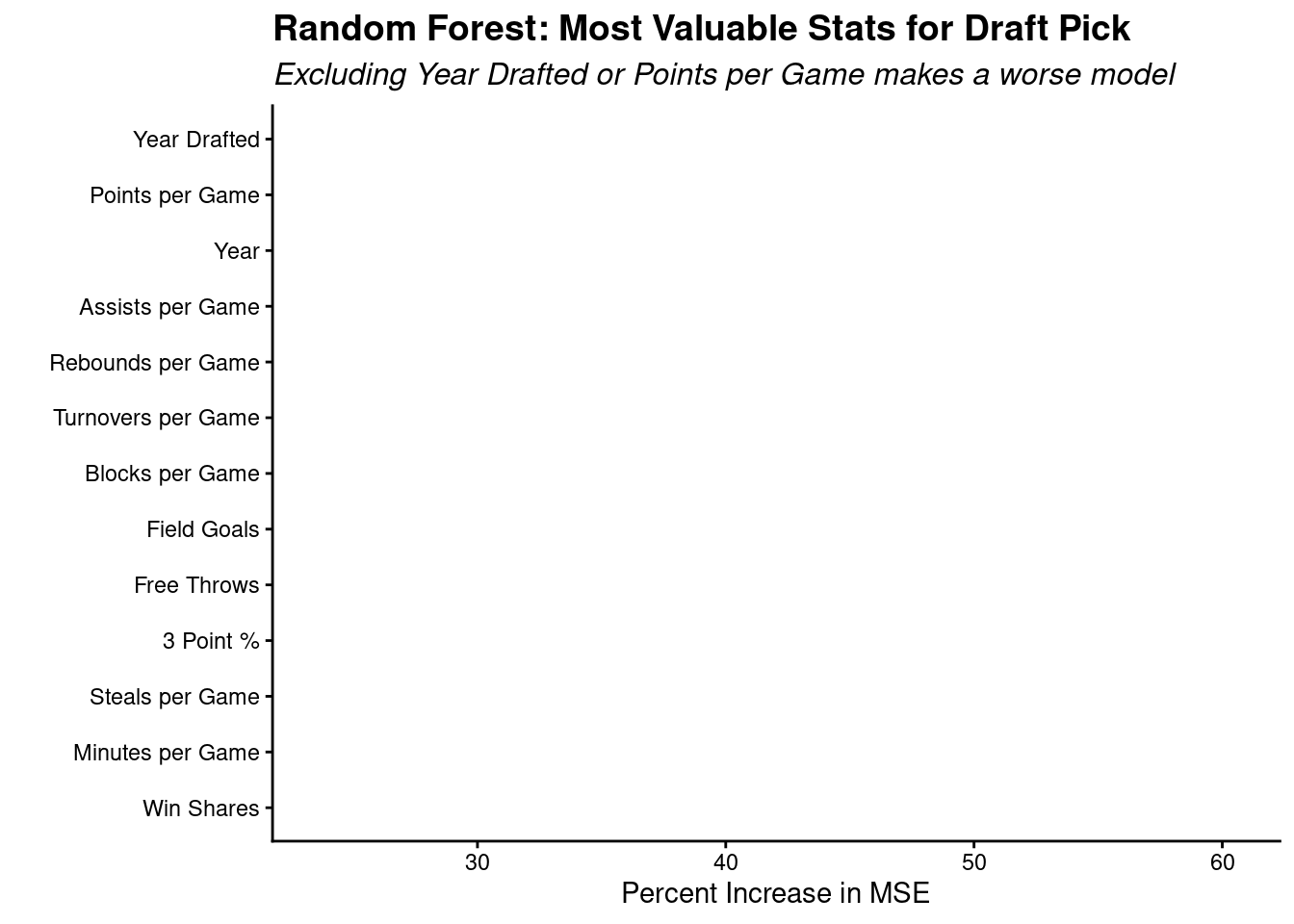
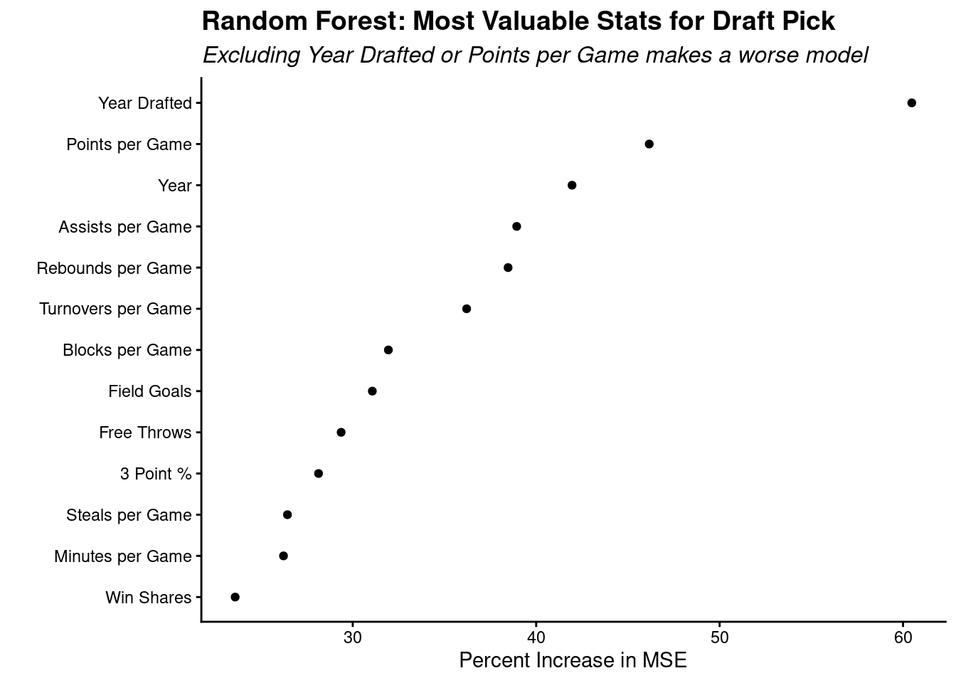
We also created a random forest to explore the relationship between variables related to drafting and the percentage error in picking the right player.

The percentage increase in MSE measures how much the prediction error increases if a variable is removed. The higher the MSE, the more important that variable is, such as points per game and assists per game, to name a few.

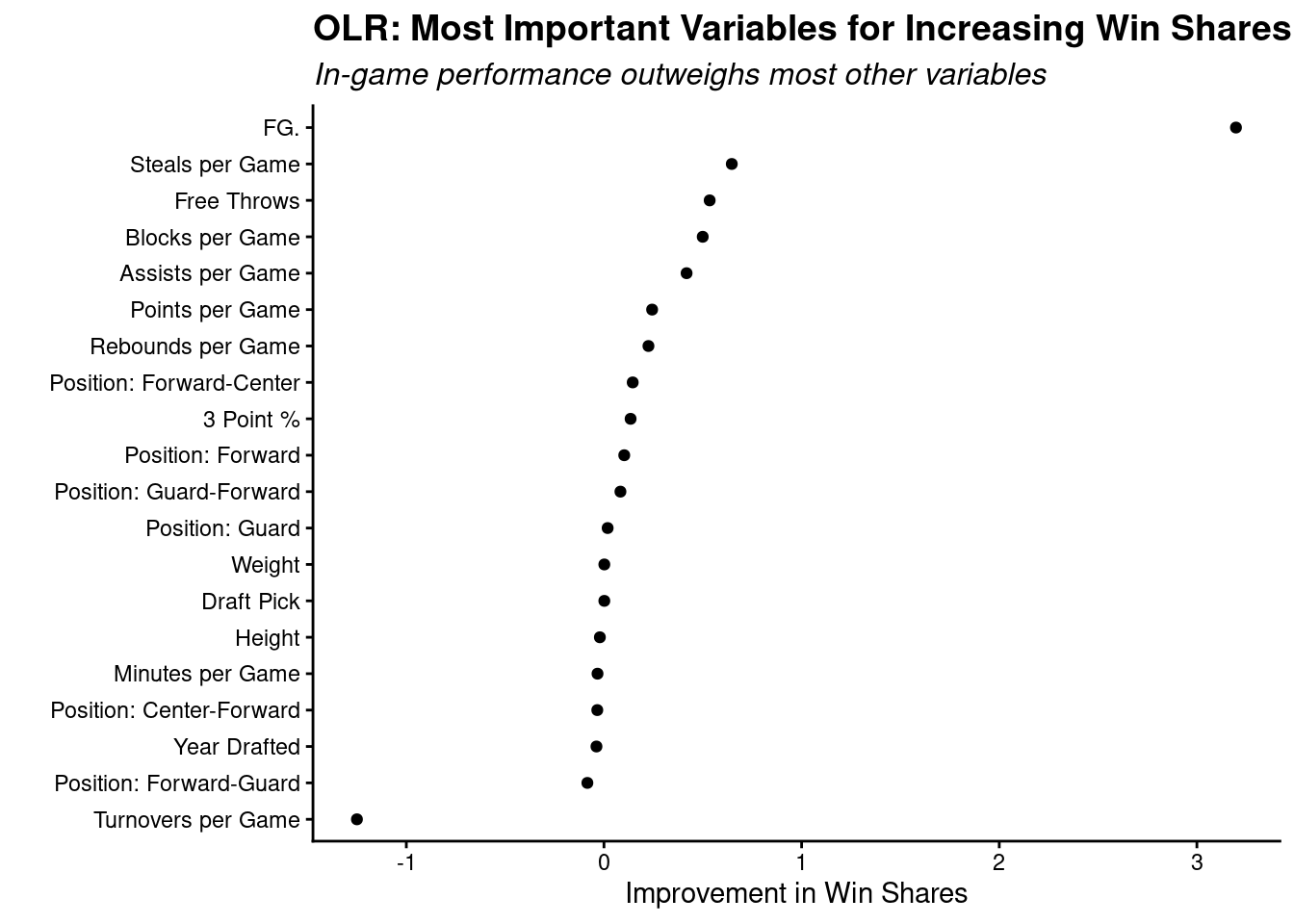
We also created an ordinary linear regression model (OLR) to explore relationships between various WNBA stats and Win Shares in more detail.

This plot illustrates the importance of different statistical categories in relation to win shares. The further to the right a category is, the better an improvement in that category does to a player’s win shares. Meaning, a one unit increase in a player’s field goal percentage has a dramatically positive effect on that player’s win shares. The inverse is true for turnovers per game.

Interpretations

According to the data that we collected, it appears that the pick that a player was selected at has an influence over the future success of that player. The player selected first overall tends to have an outsized level of success, with fewer wins generated by the 2nd through 6th picks. There is a drop of nearly two full win shares on average between first overall picks and those taken anywhere in the top six, and that gap continues to widen as selections move deeper into the draft. Players taken between seventh and fifteenth average just over one win share per season, while undrafted players who make a roster average just 0.6. The relationship is real but it is worth noting that it functions more as a proxy for talent level than as a causal mechanism. Being picked first does not make a player better; it reflects that evaluators already believed they were.

That said, draft position explains only about ten percent of the variation in win shares when modeled on its own alongside height and weight. Physical attributes, despite their intuitive appeal as predictors, turn out to have very limited standalone power. Height carries a small positive signal, taller players tend to accumulate more win shares in part because the center and forward positions naturally generate more rebounds and blocks, but weight adds almost nothing once height is accounted for. The physical model as a whole leaves ninety percent of the outcome unexplained.

The performance statistics model tells a far more complete story. Points per game, rebounds per game, assists per game, blocks per game, steals per game, field goal percentage and free throw percentage together explain roughly 74 percent of win shares variance in a standard linear model, and a random forest using the same inputs pushes that figure to 76 percent. Scoring volume is the single most important factor by a wide margin, accounting for nearly 64 percent of the random forest’s predictive power on its own. But shooting efficiency amplifies or diminishes that volume in ways that matter enormously. A player scoring fifteen points per game on 50 percent shooting generates substantially more value than the same volume on 38 percent.

The most counterintuitive finding is the role of turnovers. Of all the variables in the model, turnovers per game carry the largest negative coefficient, sitting at nearly negative one full win share per turnover per game. That means a single additional turnover per game costs a player roughly as much in win shares as a steal or an assist is worth in the positive direction. Players who protect the ball are quietly among the most valuable contributors in the league regardless of how prominently they appear in the box score.

Answer to Question

The answer to the original question is that on-court production is what drives success in the WNBA, and the specific combination of scoring efficiently, distributing the ball, defending actively and limiting turnovers separates the most impactful players from the rest. Physical size and draft pedigree provide a foundation, but they account for a small fraction of what determines how much a player actually contributes once the game is being played. The five players with the highest career win shares in our dataset, Tamika Catchings, Nneka Ogwumike, Diana Taurasi, Sylvia Fowles and Lauren Jackson, all share one characteristic above any other. They were relentless producers who made good decisions with the ball, and they did it consistently across many seasons.